Lightcurve observations of fast rotating asteroids

Short period lightcurve observations are complicated by the fact that, to obtain a usable signal-to-noise ratio, it is generally necessary to integrate on the target object for periods of time that are comparable to the lightcurve period itself. Here we describe how the finite integration time affects the observed lightcurve.

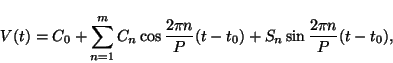
We assume that the asteroid lightcurve is periodic and its shape does not change during the observed interval. The flux of light (V, expressed in linear units) reduced to the unit geocentric and heliocentric distances and to some consistent phase angle, is a periodic function of time (t). This function can be described as a Fourier series

where C₀ is the mean reduced light flux, C_n and S_n are the Fourier coefficients of the n-th order, P is the period, and t₀ is the zero-point time (epoch). The series is truncated at the highest significant order (m).

The amplitude of the n-th harmonic is

Hereafter we take t₀=0.
The light integrated during the interval is

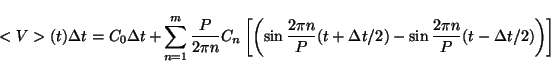
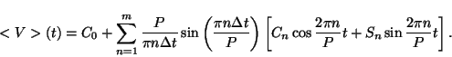
The integrated lightcurve <V> is again a Fourier series

This shows that a Fourier analysis method, like that developed by Harris et al. (1989), can be used for analysis of a lightcurve of any period observed with any integration time. A problem may arise, however, with an interpretation of obtained results. If the integration time () is not much less than the period, then the distortion (smoothing) of the lightcurve shape may lead to a situation where a reconstruction of the true lightcurve shape or even a period solution are impossible.

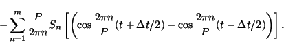
The integrated lightcurve doesn't have the same shape as the real lightcurve; its Fourier coefficients are the Fourier coefficients of the true lightcurve multiplied by factors

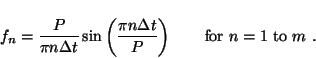
The right side of Eq. 5 has a form , where . For , for each n; i.e., no apparent distortion occurs when is much less than P. If f_n=0 (occurs when is integer), then the n-th order Fourier coefficients of the true lightcurve cannot be derived from the integrated lightcurve; the n-th harmonic is completely smoothed out by the integration.

An important question is what is the optimum integration time needed to best derive the lightcurve period. To obtain a high signal-to-noise ratio (S/N), a long integration time is needed. On the other hand, an amplitude of the integrated lightcurve's second harmonic (which is the strongest harmonic in most asteroid lightcurves) decreases with the integration time increasing from 0 to P/2 (see Eq. 5), thus the gain in S/N is reduced by the decrease of the detected amplitude. Assuming that S/N is proportional to (valid in a lower part of the dynamic range of well-designed observing systems), the optimum integration time for a detection of the second harmonic equals to 0.185 P (for which value the function reaches a maximum). For example, a 1-min rotation period can be best detected with an integration time of 11 seconds. An integration time greater than 0.185 P gives a lower integrated 2nd harmonic's signal-to-noise ratio and, since it smoothes the lightcurve, is definitely not recommended.

When an asteroid with an unknown rotation period is observed, it is naturally impossible to choose the best integration time before the observations are made. Considering that a period as short as a few minutes has been found for a small NEA (see below), it is reasonable to use integration times not greater than a few tens of seconds for similar asteroids. Of course, to obtain a reasonable S/N with such short integration times, the use of a relatively large telescope, high sensitivity CCD and even observing unfiltered are required.