MATLAB script for 3D visualizing geodata on a rotating globe: MANUAL
This is a user's guide to a free Matlab package rotating_3d_globe.zip.
To have an idea of images and animations that can be produced, have a look at the package website:
http://www.asu.cas.cz/~bezdek/vyzkum/rotating_3d_globe/.
It was our intention to prepare this package so that it can be used in a "copy and paste" style of programming.
More eloquently: "Copy, paste and quickly modify according to your needs."
♣ First download the package rotating_3d_globe.zip, unpack it
and add the '.../rotating_3d_globe/bin_geoid_3d' subfolder to your Matlab path.
This package contains also the data for the lower resolution images.
♣ For high resolution images, download data_high_resolution.zip (122 MB) separately.
To produce 3D images based on these data, you will need 4 GB of RAM memory.
♣ To create videos in compressed formats WMV, MP4, xvid AVI, download, install and add to your Matlab path: ffmpeg.
Adding the package to the Matlab search path
Modify and put the following line to your Matlab script or to your startup.m file:
addpath('REPLACE_BY_YOUR_PARTICULAR_FOLDER/rotating_3d_globe/bin_geoid_3d');
Copy some example code from the section
Matlab scripts for all the examples
of the package website and paste the copied code into your Matlab command window, possibly press Enter.
First the data should be read from a file and then a figure with the graph should open.
Finally the output image or animation should be produced and saved to your current Matlab folder.
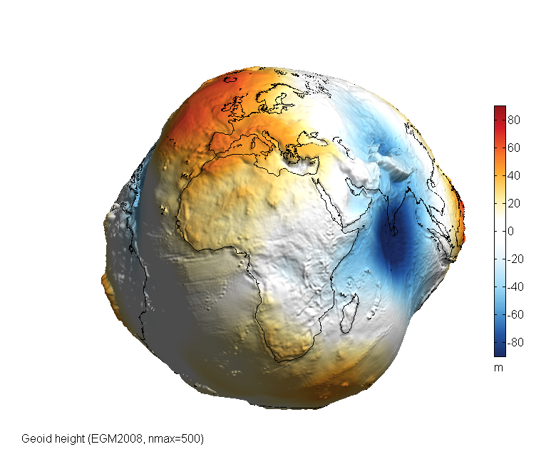
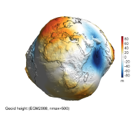
Let's take the first example: Geoid height on 3D globe.
Copy and paste the code for loading the data:
  %% Selection of geopotential model and computation/loading of the grid values
  model='egm2008';  %nmax=2190
  nmax=500;
  % Computation of grid for the selected geopotential functional
  [lond,latd,gh]=compute_geopot_grids(model,nmax,'functional','gh');
If you use the code for the first time, there will be some time needed to compute the EGM2008 grid,
next time this computed grid will be loaded quickly.
The response in the Matlab command window should be something like:
  -------------------------------
  Model: egm2008, nmax=500, half-wave: 40 km
  Grid step: 0.167 deg = 10 arcmin = 18.5 km
  Compute_geopot_grids: geoid heights (m)
  Normal field was subtracted.
  Number of points: 2334960 = 2.3 mil = 0.0 mld
  Time of computation: 4 sec = 0.1 min
  Saved file: grid_egm2008_500_gh_010m_subtr1.mat
Now try to produce the 3D graph, copy and paste the following code:
  %% Geoid height in 3D as PNG image
  rotating_3d_globe(lond,latd,gh,'coastlines',1,...
    'exaggeration_factor',1.3e4,'radius',6378e3,'units','m',...
    'graph_label',...
    sprintf('Geoid height (%s, nmax=%d)',upper(model),nmax),...
    'clbr_limits',[-90 90],'clbr_tick',-100:20:100,...
    'cptcmap_pm','BlueWhiteOrangeRed',...
    'preview_figure_visible',1,...
    'window_height',650);
Your Matlab should open a figure with the graph; at the same time a png image is saved to the harddisk.
|

|
In the Matlab command line, a message should be displayed:
  Function: ROTATING_3D_GLOBE
  Elevation data:  min=-106, max=86.7
  Preview PNG image has been created:
     rotating_3d_globe_preview_Geoid_height_EGM2008_nmax500_BlueWhiteOrangeRed_px0650.png
Each time the function rotating_3d_globe is invoked, it outputs the maximum and minimum values of the elevation data,
the name of the created png image is also reported.
If you encounter a problem, look at Troubleshooting section or contact me directly:
 . .
This chapter provides an explanation of how to use the main function of the package
rotate_3d_globe.
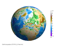
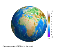
We demonstrate its basic usage on simple examples using the Earth topography data,
which we chose because the topography of our home planet is familiar to all of us.
Let's take the Earth topography data with the grid step of ten arcminutes.
First load the data (which are provided in the package):
  %% Selection of Earth topographical data: 1 degree grid
  model='ETOPO2_010arcmin';
  fprintf('Loading Earth data: %s\n',model);
  load (model);
Now produce a simple 3D graph:
  %% Earth topography: getting started
  rotating_3d_globe(lond_etopo2,latd_etopo2,elev_etopo2_km,...
     'radius',6378,'units','km');
|
|
The first three arguments of the function rotating_3d_globe
are always the same:
rotating_3d_globe(lond,latd,elev,'radius',R,'units','km');
where lond is vector of N longitudes
and latd a vector of M latitudes (both in degrees);
the third parameter elev is an M×N matrix with the elevation data.
Then there follow two other arguments, 'radius' defines the radius R,
to which the elev data are added and then visualized;
the argument 'units' is used as the colorbar label.
Do not forget to define an appropriate value for the 'radius', onto which your elevation
data will be superposed for the surface plot,
otherwise you get rather strange images!
  %% Earth topography: omission of specifying the radius
  model='ETOPO2_010arcmin'; load (model);
  rotating_3d_globe(lond_etopo2,latd_etopo2,elev_etopo2_km);
|
|
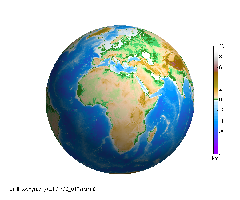
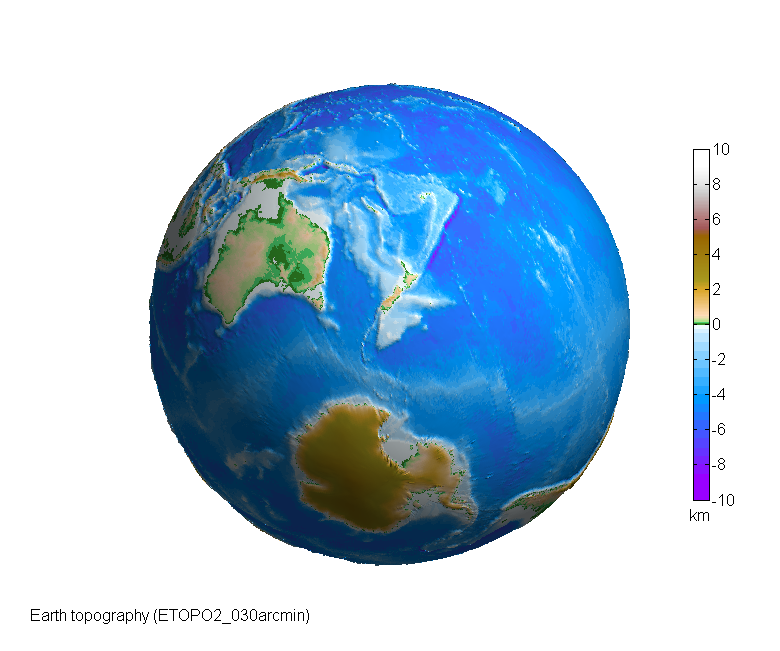
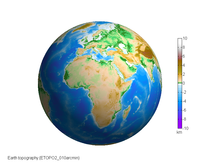
To add a descriptive text and to get nicer image colouring and an appropriate colorbar, use:
  %% Earth topography: label, larger image size and colorbar limits
  model='ETOPO2_010arcmin'; load (model);
  rotating_3d_globe(lond_etopo2,latd_etopo2,elev_etopo2_km,...
     'radius',6378,'units','km',...
     'cptcmap_pm','GMT_globe',...
     'clbr_limits',[-10 10],'clbr_tick',-10:2:10,...
     'graph_label',sprintf('Earth topography (%s)',model),...
     'window_height',650);
|
|
where the optional arguments modify the output:
'graph_label' is followed by the string for the label;
'cptcmap_pm' determines the color palette used (see Color Palette Tables (.cpt) for Matlab);
for the Earth topography data to be represented reliably it is indispensable to use a specific colour scale (here "GMT_globe.cpt"),
with other data one is free to choose arbitrary colour scale, see Section 6.1. Choosing and editing a colour scale;
'clbr_limits' and 'clbr_tick' specify the colorbar limits and ticks;
finally 'window_height' defines the figure window size, which is then used also for the png image produced.
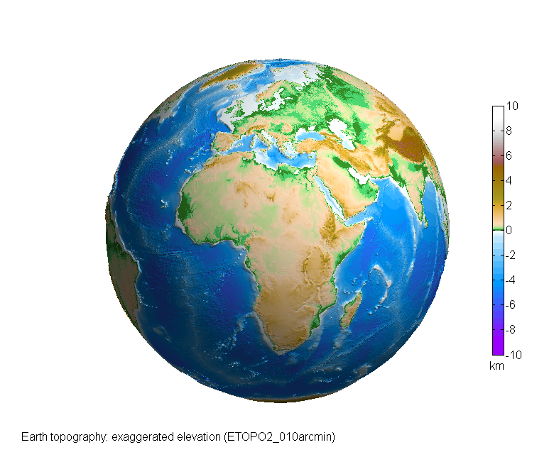
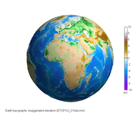
In the case of Earth topography data in ETOPO2, the elev variations are under 10 kilometres,
thus relative to the Earth radius 6378 km they are virtually invisible in the scale of our small globe.
To make the 3D visualization more illustrative, some artificial exaggeration may be added:
  %% Earth topography: slight exaggeration of elevation
  model='ETOPO2_010arcmin'; load (model);
  rotating_3d_globe(lond_etopo2,latd_etopo2,elev_etopo2_km,...
     'exaggeration_factor',13,'radius',6378,'units','km',...
     'cptcmap_pm','GMT_globe',...
     'clbr_limits',[-10 10],'clbr_tick',-10:2:10,...
     'graph_label',...
     sprintf('Earth topography: exaggerated elevation (%s)',model),...
     'window_height',650);
|
|
A slight exaggeration is rather impressive with more detailed data and larger figure sizes, as e.g. in
our high resolution example image
of Earth topography, its Matlab code is
here
on the package website.
On the contrary, if one needs only an image/animation of global data projected in colours on a perfect sphere,
it is possible to define the spherical surface of constant radius and add the scalar elev data
only as information about the colour:
  %% Earth topography: colour scale on a perfect sphere
  model='ETOPO2_010arcmin'; load (model);
  grid_of_ones=ones(size(elev_etopo2_km));  %unit sphere
  rotating_3d_globe(lond_etopo2,latd_etopo2,grid_of_ones,...
     'units','km',...
     'elev_colour',elev_etopo2_km,...
     'cptcmap_pm','GMT_globe',...
     'clbr_limits',[-10 10],'clbr_tick',-10:2:10,...
     'graph_label',...
     sprintf('Earth topography: on perfect sphere (%s)',model),...
     'window_height',650);
|

|
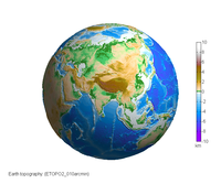
It is possible to supply geographic coordinates of the view point, see this example:
  %% Earth topography: changing the view point
  % geographic coordinates of view point: Himalaya
  latd_view_point=28;  %latitude (deg)
  lond_view_point=87;  %longitude (deg)

  model='ETOPO2_010arcmin'; load (model);
  rotating_3d_globe(lond_etopo2,latd_etopo2,elev_etopo2_km,...
     'exaggeration_factor',13,'radius',6378,'units','km',...
     'cptcmap_pm','GMT_globe',...
     'clbr_limits',[-10 10],'clbr_tick',-10:2:10,...
     'graph_label',sprintf('Earth topography: (%s)',model),...
     'azimuth',90+lond_view_point,'elevation',latd_view_point,...
     'window_height',650);
|
|
Zooming can be easily implemented by changing the camera view angle (in degrees).
Try several values for view_angle: 3 corresponds to regional view, 1 or 2 gets you more closer.
  %% Earth topography: changing the view point, zoom in
  % geographic coordinates of view point: Himalaya
  latd_view_point=28;  %latitude (deg)
  lond_view_point=87;  %longitude (deg)

  % Zooming can be implemented by changing the camera view angle (in degrees).
  % Try values: 3 corresponds to regional view, 1 or 2 gets you more closer
  view_angle=3;

  model='ETOPO2_010arcmin'; load (model);
  %model='ETOPO2_004arcmin'; load (model);
  rotating_3d_globe(lond_etopo2,latd_etopo2,elev_etopo2_km,...
     'exaggeration_factor',13,'radius',6378,'units','km',...
     'cptcmap_pm','GMT_globe',...
     'clbr_limits',[-10 10],'clbr_tick',-10:2:10,...
     'graph_label',sprintf('Earth topography: (%s)',model),...
     'preview_figure_visible',1,...
     'azimuth',90+lond_view_point,'elevation',latd_view_point,...
     'view_angle',view_angle,...
     'window_height',650);
|
|
This example is the same as the previous, only we choose data with finer resolution spatial resolution of 4 arcmin:
model='ETOPO2_004arcmin'; load (model);
Because working with 4-arcmin data is more computationally intensive,
to speed up the generation of the png image, it is better to let the figure window be invisible:
'preview_figure_visible',0,...
You can make your figure window again visible by typing:
set(gcf,'visible','on')
The default behaviour is to show the figure windows with png preview images and to hide the animation windows.
  %% Earth topography: changing the view point, zoom in
  % geographic coordinates of view point: Himalaya
  latd_view_point=28;  %latitude (deg)
  lond_view_point=87;  %longitude (deg)

  % Zooming can be implemented by changing the camera view angle (in degrees).
  % Try values: 3 corresponds to regional view, 1 or 2 gets you more closer
  view_angle=3;

  % model='ETOPO2_010arcmin'; load (model);
  model='ETOPO2_004arcmin'; load (model);
  rotating_3d_globe(lond_etopo2,latd_etopo2,elev_etopo2_km,...
     'exaggeration_factor',13,'radius',6378,'units','km',...
     'cptcmap_pm','GMT_globe',...
     'clbr_limits',[-10 10],'clbr_tick',-10:2:10,...
     'graph_label',sprintf('Earth topography: (%s)',model),...
     'preview_figure_visible',0,...
     'azimuth',90+lond_view_point,'elevation',latd_view_point,...
     'view_angle',view_angle,...
     'window_height',650);
|
|
Modifying the code below, you can plot the position and name of your hometown or other point of interest.
  %% Earth topography: changing the view point, plot a point
  % geographic coordinates of view point: Prague, Czech Republic
  latd_view_point=50;  %latitude (deg)
  lond_view_point=14.5;  %longitude (deg)

  model='ETOPO2_010arcmin'; load (model);
  [hc,hlab,name_png]=...
     rotating_3d_globe(lond_etopo2,latd_etopo2,elev_etopo2_km,...
     'exaggeration_factor',13,'radius',6378,'units','km',...
     'cptcmap_pm','GMT_globe',...
     'clbr_limits',[-10 10],'clbr_tick',-10:2:10,...
     'graph_label',sprintf('Earth topography: (%s)',model),...
     'azimuth',90+lond_view_point,'elevation',latd_view_point,...
     'window_height',650);

  % Plot and label the point
  % we need to know 'exaggeration_factor' and 'radius' to place the point
  %  on the displayed surface
  exaggeration_factor=13;
  radius=6378;
  elev_view_point=interp2(lond_etopo2,latd_etopo2,elev_etopo2_km,...
                          lond_view_point,latd_view_point);
  r=radius/exaggeration_factor+elev_view_point;
  [xx,yy,zz]=sph2cart(lond_view_point/rad,latd_view_point/rad,r);
  hold on
  plot3(xx,yy,zz,'r.','MarkerSize',13)
  text(xx,yy,zz,' Prague','fontSize',12,'color','red','FontWeight','bold')
  eval(sprintf('print -dpng -r0 %s;',name_png)); %save the figure again
|
|
As in the example above using 4-arcmin Earth topography data,
to produce such a detailed image
it is faster to use an invisible figure window.
  %% Earth topography: changing the view point, zoom in, plot a point
  % geographic coordinates of view point: Prague, Czech Republic
  latd_view_point=50;  %latitude (deg)
  lond_view_point=14.5;  %longitude (deg)

  % Zooming can be implemented by changing the camera view angle (in degrees).
  % Try values: 3 corresponds to regional view, 1 or 2 gets you more closer
  view_angle=2;

  model='ETOPO2_004arcmin'; load (model);
  [hc,hlab,name_png]=...
     rotating_3d_globe(lond_etopo2,latd_etopo2,elev_etopo2_km,...
     'exaggeration_factor',13,'radius',6378,'units','km',...
     'cptcmap_pm','GMT_globe',...
     'clbr_limits',[-10 10],'clbr_tick',-10:2:10,...
     'graph_label',sprintf('Earth topography: (%s)',model),...
     'preview_figure_visible',0,...
     'azimuth',90+lond_view_point,'elevation',latd_view_point,...
     'view_angle',view_angle,...
     'window_height',650);

  % Plot and label the point
  % we need to know 'exaggeration_factor' and 'radius' to place the point
  % on the displayed surface
  exaggeration_factor=13;
  radius=6378;
  elev_view_point=interp2(lond_etopo2,latd_etopo2,elev_etopo2_km,...
                          lond_view_point,latd_view_point);
  r=radius/exaggeration_factor+elev_view_point;
  [xx,yy,zz]=sph2cart(lond_view_point/rad,latd_view_point/rad,r);
  hold on
  plot3(xx,yy,zz,'r.','MarkerSize',13)
  text(xx,yy,zz,' Prague','fontSize',12,'color','red','FontWeight','bold')
  eval(sprintf('print -dpng -r0 %s;',name_png)); %save the figure again
|
|
To include coastlines and country boundaries, simply add them as optional arguments:
     'coastlines',1,...
     'countries',1,...
We use the data downloaded from
http://www.naturalearthdata.com/.
  %% Earth topography: zoom in, coastlines and country boundaries
  % geodetic coordinates of view point: Potsdam, Germany
  latd_view_point=52;
  lond_view_point=13;

  % Zooming can be implemented by changing the camera view angle (in degrees).
  % Try values: 3 corresponds to regional view, 1 or 2 gets you more closer
  view_angle=2;

  model='ETOPO2_004arcmin'; load (model);
  rotating_3d_globe(lond_etopo2,latd_etopo2,elev_etopo2_km,...
     'exaggeration_factor',13,'radius',6378,'units','km',...
     'coastlines',1,...
     'countries',1,...
     'cptcmap_pm','GMT_globe',...
     'clbr_limits',[-10 10],'clbr_tick',-10:2:10,...
     'graph_label',sprintf('Earth topography: (%s)',model),...
     'preview_figure_visible',0,...
     'azimuth',90+lond_view_point,'elevation',latd_view_point,...
     'view_angle',view_angle,...
     'window_height',650);
|
|
To add grid lines to the Earth's surface plot, one inserts the following line among the list of optional arguments:
'grid',1,...
The default values for the step in longitudes is 60 deg, in latitude 30 deg, these can be modified:
   'grid_lond',30,...
   'grid_latd',15,...
For the previous example showing data on a coloured perfect sphere, we can add the grid lines in this way:
  %% Earth topography: colour scale on a perfect sphere + grid lines
  model='ETOPO2_010arcmin'; load (model);
  grid_of_ones=ones(size(elev_etopo2_km));  %unit sphere
  rotating_3d_globe(lond_etopo2,latd_etopo2,grid_of_ones,...
    'units','km',...
    'elev_colour',elev_etopo2_km,...
    'cptcmap_pm','GMT_globe',...
    'clbr_limits',[-10 10],'clbr_tick',-10:2:10,...
    'grid',1,...
    'graph_label',...
    sprintf('Earth topography: on perfect sphere + grid lines (%s)',model),...
    'window_height',650);
|

|
The usage of the function
rotating_3d_globe
is the same as for still images, in order to produce animations, several optional arguments are needed:
'clbr_anim',1,'clbr_reduce',0.4,...
parameter clbr_anim sets whether (1) or not (0) the colorbar is produced in the animation window,
clbr_reduce sets the size reduction of the colorbar (the default value is 0.6).
If you want an animated gif to be produced:
'anim_gif',1,...
Then
anim_angle
sets the ending angle for the animated rotation (in degrees; full angle 360 deg, smaller angle is used for debugging, as here 36 deg).
'anim_angle',36,'time_for_360deg',42,'fps',1,...
time_for_360deg is the time for the animation to make a full rotation of 360 deg (in seconds)
and fps defines 'frames per second' of the video.
In this example we choose 1 fps, which produces jerky rotational motion;
on the other hand, all the details around the globe could be presented and the file size of the produced gif is small
(200 kB with this 350-pixel gif for the 36-deg angle, therefore cca 2 MB for the full rotation of 360 degrees).
%% Earth topography in 3D as animated GIF: 36-degree segment, 1 fps
model='ETOPO2_010arcmin'; load (model);
rotating_3d_globe(lond_etopo2,latd_etopo2,elev_etopo2_km,...
   'exaggeration_factor',13,'radius',6378,'units','km',...
   'cptcmap_pm','GMT_globe',...
   'clbr_limits',[-10 10],'clbr_tick',-10:2:10,...
   'graph_label',sprintf('Earth topography: (%s)',model),...
   'preview_figure_visible',0,...
   'clbr_anim',1,'clbr_reduce',0.4,...
   'anim_gif',1,...
   'anim_angle',36,'time_for_360deg',42,'fps',1,...
   'window_height',350);
|
|
We set a higher frame rate, 10 fps, which produces smoother rotation, still finite rotational steps are discernible.
The file is 10 times bigger than with 1 fps.
'anim_angle',36,'time_for_360deg',42,'fps',10,...
|
|
Setting the frame rate of 20 fps and higher results in smooth motion (cf. http://en.wikipedia.org/wiki/Frame_rate).
The problem here is the "flickering" or "twinkling" of the fine details in the animation; this problem is resolved in the following paragraph.
'anim_angle',36,'time_for_360deg',42,'fps',20,...
|
|
If the represented elevation data contain fine details, then a high-rate animation of fps>10 creates an unpleasant flickering of these details,
as they change their position from one frame to another. We found a solution in using an intermediate larger window:
'window_height_intermediate',700,...
Each frame is first produced with larger size, which is then slightly smoothed (in fact, this is an anti-aliasing filter) and then its size is reduced
to the final dimensions. A factor of 2 or 3 for larger window seems satisfactory; so e.g. to obtain this 350-px animation, an intermediate window of 700 px was used.
The rotational motion is now smooth and with an acceptable level of flickering.
  %% Earth topography as animated GIF: 36-deg segment, 20 fps, smoothed
  model='ETOPO2_010arcmin'; load (model);
  rotating_3d_globe(lond_etopo2,latd_etopo2,elev_etopo2_km,...
     'exaggeration_factor',13,'radius',6378,'units','km',...
     'cptcmap_pm','GMT_globe',...
     'clbr_limits',[-10 10],'clbr_tick',-10:2:10,...
     'graph_label',sprintf('Earth topography: (%s)',model),...
     'preview_figure_visible',0,...
     'clbr_anim',1,'clbr_reduce',0.4,...
     'anim_gif',1,...
     'anim_angle',36,'time_for_360deg',42,'fps',20,...
     'window_height_intermediate',700,...
     'window_height',350);
|

|
This example illustrates all the features of producing an animated GIF described so far.
To reduce the size of the file which should comprise the full animation angle of 360 deg, we chose it to be of "thumbnail" size 110 px.
To avoid flickering, the size of intermediate window was set to be 330 px.
Such a small image size allows one to decrease the rotation rate without making the motion too jerky, so we set
fps to 7. File size of this example: 2 MB.
  %% Earth topography in 3D as animated GIF: full revolution, smooth motion
  model='ETOPO2_030arcmin'; load (model);
  rotating_3d_globe(lond_etopo2,latd_etopo2,elev_etopo2_km,...
     'exaggeration_factor',13,'radius',6378,'units','km',...
     'cptcmap_pm','GMT_globe',...
     'clbr_limits',[-10 10],'clbr_tick',-10:2:10,...
     'preview_figure_visible',0,...
     'clbr_anim',0,...
     'anim_gif',1,...
     'anim_angle',360,'time_for_360deg',42,'fps',7,...
     'window_height_intermediate',330,...
     'window_height',110);
|
|
After the removal of flickering, the smoothed 36-deg portion of 20-fps animated gif has the size of 3.8 MB.
A gif file with the full 360-deg rotation would have 38 MB, which is too much for use in presentations etc.
To reduce the file size, smaller dimensions and fps may be used as in the previous point.
Another possibility is to use a compressed video file instead of an animated gif,
which has a comparable quality and significantly smaller size (14 MB in this example).
Other choices for
video_format are 'wmv','mp4','xvid' for compressed video files,
and 'uncomp' to save the animation in an uncompressed Matlab avi video file.
  %% Earth topography in 3D as video files: WMV, MP4, xvid AVI
  model='ETOPO2_010arcmin'; load (model);
  rotating_3d_globe(lond_etopo2,latd_etopo2,elev_etopo2_km,...
     'exaggeration_factor',13,'radius',6378,'units','km',...
     'cptcmap_pm','GMT_globe',...
     'clbr_limits',[-10 10],'clbr_tick',-10:2:10,...
     'graph_label',sprintf('Earth topography: (%s)',model),...
     'preview_figure_visible',0,...
     'clbr_anim',1,'clbr_reduce',0.4,...
     'video_format','wmv',...
     'anim_gif',1,...
     'anim_angle',360,'time_for_360deg',42,'fps',20,...
     'window_height_intermediate',700,...
     'font_size',27,...
     'window_height',350);
|
|
Using the optional argument:
'anim_gif',2,...
a folder is created, where the png images used for producing the animated gif are stored.
Each png image has finer colour transitions due to higher colour depth of 24 bits compared to 8 bits of animated gifs.
  %% Earth topography in 3D animation: PNG files for slideshow
  model='ETOPO2_010arcmin'; load (model);
  rotating_3d_globe(lond_etopo2,latd_etopo2,elev_etopo2_km,...
     'exaggeration_factor',13,'radius',6378,'units','km',...
     'cptcmap_pm','GMT_globe',...
     'clbr_limits',[-10 10],'clbr_tick',-10:2:10,...
     'graph_label',sprintf('Earth topography: (%s)',model),...
     'preview_figure_visible',0,...
     'clbr_anim',1,'clbr_reduce',0.4,...
     'anim_gif',2,...
     'anim_angle',360,'time_for_360deg',36,'fps',1,...
     'window_height',500);
|
|
rotating_3d_globe_Earth_topography
_ETOPO2_010arcmin_px0500
_angle360_fps1_GMT_globe.zip
|
To visualize a gravity field model, we need a grid of the required geopotential functional computed from the given model.
A model is defined by its harmonic coefficients (see the reference paper for details).
The harmonic coefficients are saved in mat files named after the model.
In the package, there are several models available, of different maximum resolution (stated in comments):
  %% Selection of geopotential model and computation/loading of the grid values
  % model='asu-ch-0309'; %nmax 120
  % model='itg-grace2010s'; %nmax 180
  % model='GOCO03S';  %nmax 250
  model='egm2008';  %nmax=2190
According to the spatial resolution of the model defined by its maximum degree 'nmax', the function compute_geopot_grids selects
a corresponding value for the step of the grid, also the vectors of longitudes and latitudes are output:
  model='egm2008'; nmax=500;    %selection of geopotential model
  [lond,latd,gh]=compute_geopot_grids(model,nmax,'functional','gh');
An suitable spatial resolution of the 3D image determines the necessary maximum degree 'nmax', if available for the given model, for example:
  nmax=180    grid_stepd*60 = 30 arcmin = 0.5 deg
  nmax=500    grid_stepd*60 = 10 arcmin = 0.1666... deg
  nmax=1000   grid_stepd*60 =  5 arcmin = 0.8333... deg
For small images/animations of say 110 px, a grid of 0.5 deg is sufficient (nmax=180),
for medium sized images of 300–1000 px a grid of 10 arcmin is adequate (nmax=500),
for high-resolution images presented on the package website we used 4 or 5 arcmin data (nmax equal to 1100 or 1000),
e.g.
high resolution example image
of geoid height, its Matlab code is
here.
The computation of the grid needed for the visualization is done by invoking e.g.:
   model='egm2008'; nmax=500;    %selection of geopotential model
   [lond,latd,gh]=compute_geopot_grids(model,nmax,'functional','gh');
The function
compute_geopot_grids
tests, whether the grid has already been computed and stored.
In the folder 'temp', the computed geopotential grids are stored for speeding up the execution of the function.
You may delete its contents if you wish.
We save only grids which took more than 'time_limit_to_save_grids' seconds to compute (the default is 1 sec).
We provide the user a possibility of using any of the gravity field models stored at
ICGEM website (click on 'Table of models' in the menu on the left).
The downloaded gfc file is then transformed into our internal format by typing:
icgem2mat
This function finds all the ICGEM files (*.gfc) in the current directory,
reads the geopotential coefficients and transforms them into Matlab variables for much faster loading.
The new mat file with the same name is moved into 'data_icgem' subdirectory;
the original gfc file is moved into 'data_icgem/gfc/' subdirectory.
Add the 'data_icgem' folder into your Matlab path.
The model coefficients are then loaded by typing, e.g.
load egm2008
Usage and meaning of the optional arguments was explained in Section
2. Making of 3D graphs step by step,
computation of the grid for the geoid height in the previous section.
♣
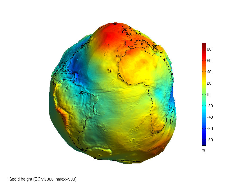
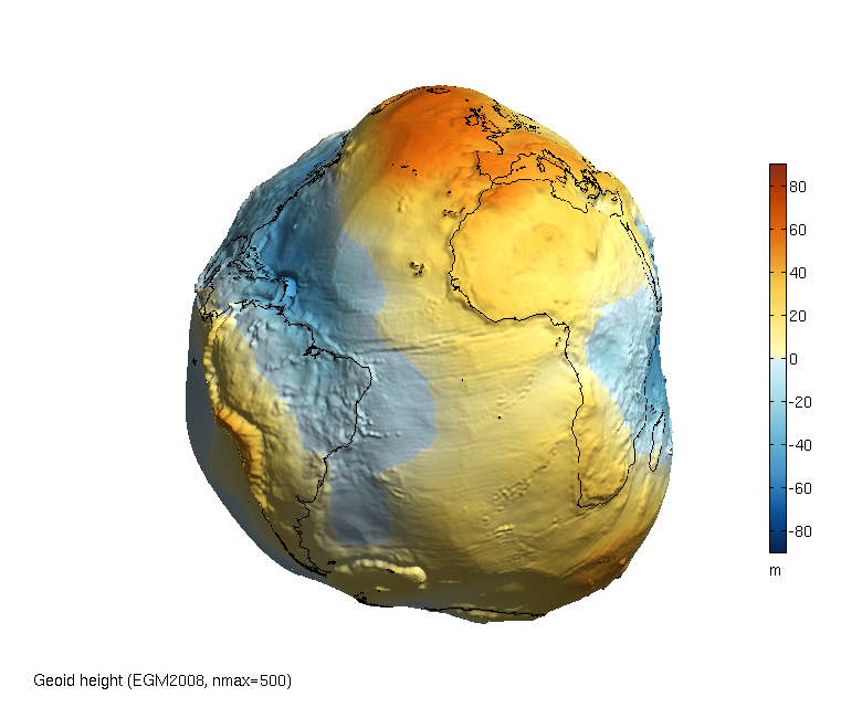
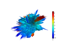
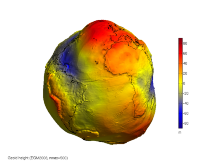
For geoid heights, a rather large exaggeration factor 1.3e4 is usually applied to greatly emphasize the difference of the Earth shape with respect
to the best fitting ellipsoid (for details, see the reference paper).
  %% Geoid height in 3D as PNG image
  model='egm2008'; nmax=500;    %selection of geopotential model
  [lond,latd,gh]=compute_geopot_grids(model,nmax,'functional','gh');
  [hc,hlab,name_png]=rotating_3d_globe(lond,latd,gh,'coastlines',1,...
     'exaggeration_factor',1.3e4,'radius',6378e3,'units','m',...
     'graph_label',...
     sprintf('Geoid height (%s, nmax=%d)',upper(model),nmax),...
     'clbr_limits',[-90 90],'clbr_tick',-100:20:100,...
     'cptcmap_pm','BlueWhiteOrangeRed',...
     'preview_figure_visible',1,...
     'window_height',650);
|
|
An example of animation that can be used e.g. in a presentation, due to its relatively small size.
A small frame rate 1 fps was taken for a medium sized window of 500 px, which produced an
animated gif
of 3.1 MB
and a
wmv compressed
animation of 2.4 MB.
  %% Geoid height in 3D as animated GIF/compressed video: 1 fps
  % jako ze to je vhodne napr. do prezentace
  model='egm2008'; nmax=500;    %selection of geopotential model
  [lond,latd,gh]=compute_geopot_grids(model,nmax,'functional','gh');
  [hc,hlab,name_png]=rotating_3d_globe(lond,latd,gh,...
     'coastlines',1,...
     'exaggeration_factor',1.3e4,'radius',6378e3,'units','m',...
     'cptcmap_pm','BlueWhiteOrangeRed',...
     'graph_label',...
     sprintf('Geoid height (%s, nmax=%d)',upper(model),nmax),...
     'clbr_limits',[-90 90],'clbr_tick',-100:20:100,...
     'preview_figure_visible',0,...
     'clbr_anim',1,'clbr_reduce',0.4,...
     'video_format','wmv',...
     'anim_gif',1,...
     'anim_angle',360,'time_for_360deg',42,'fps',1,...
     'window_height',500);
|

|
The same "thumbnail" animation as is described above in Section
3.2 for Earth topography.
.
  %% Geoid height in 3D as animated GIF: full revolution, smooth motion
  model='egm2008'; nmax=180;    %selection of geopotential model
  [lond,latd,gh]=compute_geopot_grids(model,nmax,'functional','gh');
  [hc,hlab,name_png]=rotating_3d_globe(lond,latd,gh,...
     'radius',6378e3,'units','m',...
     'exaggeration_factor',1.3e4,...
     'coastlines',1,...
     'cptcmap_pm','BlueWhiteOrangeRed',...
     'clbr_limits',[-90 90],'clbr_tick',-100:20:100,...
     'preview_figure_visible',0,...
     'clbr_anim',0,...
     'anim_gif',1,...
     'anim_angle',360,'time_for_360deg',42,'fps',7,...
     'window_height_intermediate',330,...
     'window_height',110);
|
|
This is an example of smoothly rotating geoid, whose definition and properties are described above in
Section 3.3 for Earth topography.
As above, for this smooth animation covering the full 360-deg rotation angle, with high time resolution of 20 fps,
the size of the wmv file is 13 MB, much smaller than the corresponding animated gif of 37 MB.
  %% Geoid height in 3D as video files: WMV, MP4, xvid AVI
  model='egm2008'; nmax=500;    %selection of geopotential model
  [lond,latd,gh]=compute_geopot_grids(model,nmax,'functional','gh');
  [hc,hlab,name_png]=rotating_3d_globe(lond,latd,gh,...
     'coastlines',1,...
     'exaggeration_factor',1.3e4,'radius',6378e3,'units','m',...
     'cptcmap_pm','BlueWhiteOrangeRed',...
     'graph_label',...
     sprintf('Geoid height (%s, nmax=%d)',upper(model),nmax),...
     'clbr_limits',[-90 90],'clbr_tick',-100:20:100,...
     'preview_figure_visible',0,...
     'clbr_anim',1,'clbr_reduce',0.4,...
     'video_format','wmv',...
     'anim_gif',1,...
     'anim_angle',360,'time_for_360deg',42,'fps',20,...
     'window_height_intermediate',700,...
     'font_size',27,...
     'window_height',350);
|
|
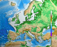
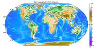
We provide the functionality of creating 2D elevation maps only as an addendum to our main 3D visualization function
compute_geopot_grids, because often it is useful to project the elevation data also to a 2D map.
Our 2D calling function
elevation_2d_map
shares the basic syntax with the 3D function compute_geopot_grids,
but in fact it serves only as a wrapper, which uses
M_Map: A mapping package for Matlab.
Usage of our 2D mapping function is fully analogous to 3D visualization function as explained above in
Section 2. Making of 3D graphs step by step.
As explained in
the section about zooming the detailed Earth topography data,
for speeding up the generation of the png file, we set the figure window as invisible.
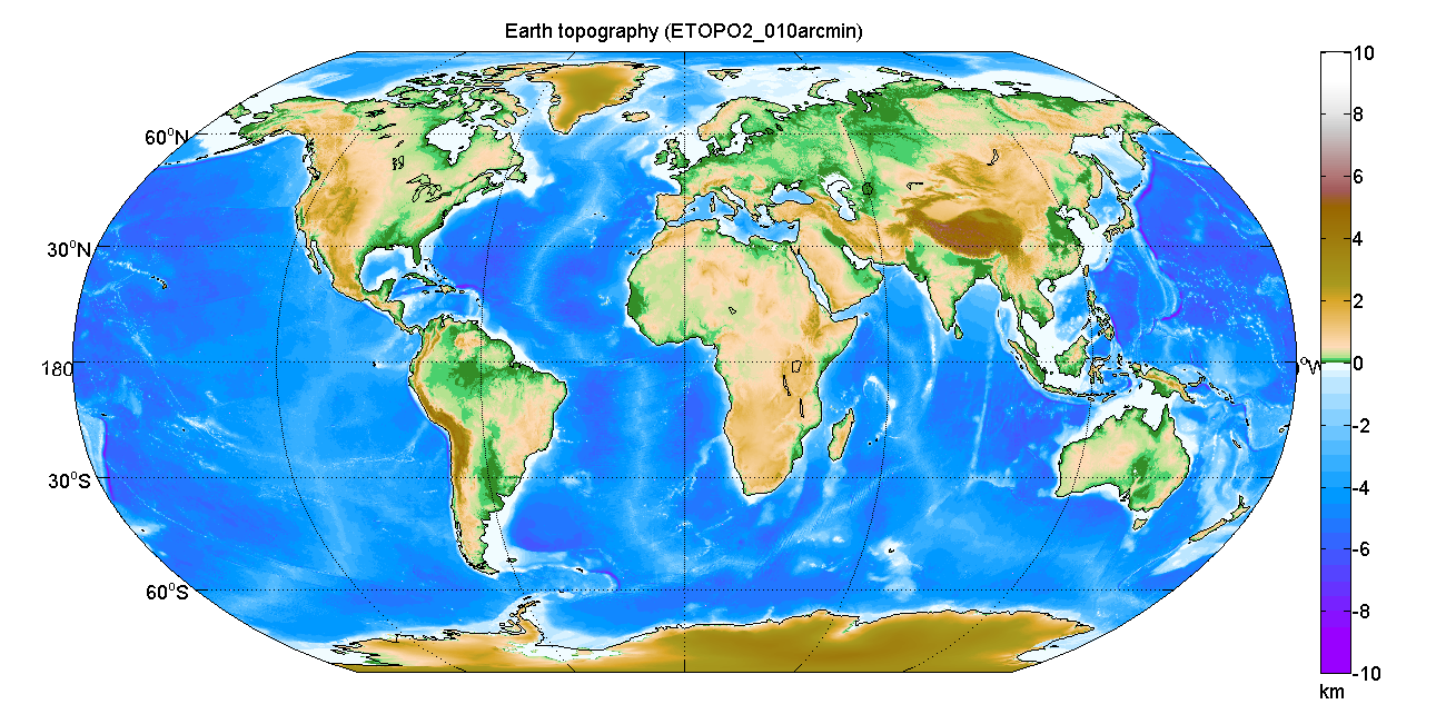
  %% Earth topography as 2D map
  model='ETOPO2_010arcmin'; load (model);
  elevation_2d_map(lond_etopo2,latd_etopo2,elev_etopo2_km,...
     'coastlines',1,...
     'units','km',...
     'graph_label',sprintf('Earth topography (%s)',model),...
     'clbr_limits',[-10 10],'clbr_tick',-10:2:10,...
     'cptcmap_pm','GMT_globe',...
     'preview_figure_visible',0,...
     'window_height',650);
|
|
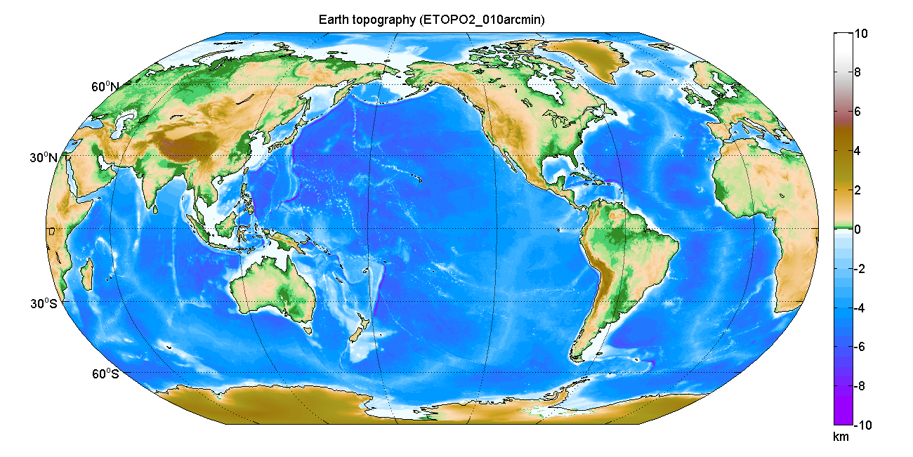
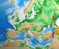
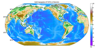
This example shows how to change the view point to the Pacific rather than to the Greenwich meridian (default).
  %% Earth topography as 2D map (centred on the Pacific)
  model='ETOPO2_010arcmin'; load (model);
  elevation_2d_map(lond_etopo2,latd_etopo2,elev_etopo2_km,...
     'map_center','Pacific',...
     'coastlines',1,...
     'units','km',...
     'graph_label',sprintf('Earth topography (%s)',model),...
     'clbr_limits',[-10 10],'clbr_tick',-10:2:10,...
     'cptcmap_pm','GMT_globe',...
     'preview_figure_visible',0,...
     'window_height',650);
|
|
All the functions in our package have a help, which could be invoked by typing 'help' or 'doc', for example
doc rotating_3d_globe
In addition to the help, you can have a look and modify the code.
Sometimes, users complain that Matlab does not produce nicely looking images with varied colour scales.
We believe that this is not true, look for example at our
high resolution example image
of Earth topography.
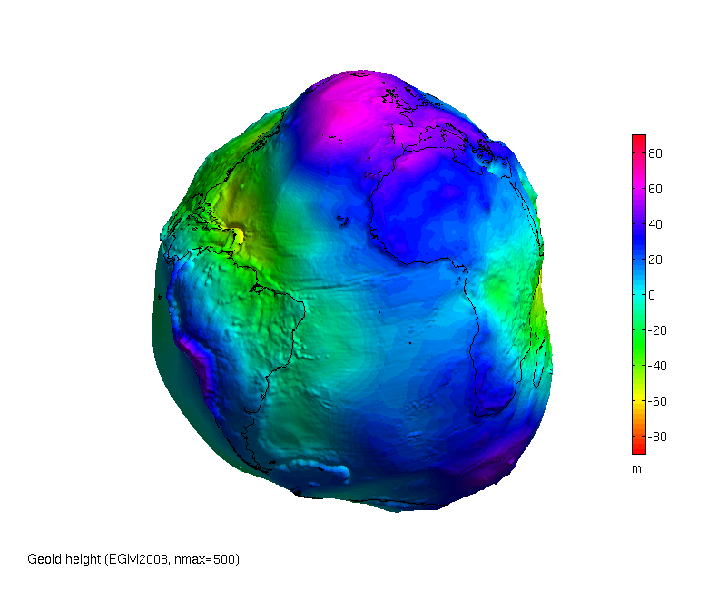
In fact, a user can quickly and easily change and edit a color scale for 2D or 3D images.
Without defining a specific colour scale, a default Matlab colormap called 'Jet' is used.
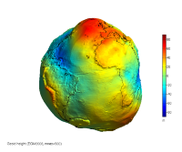
  %% Choosing and editing a colour scale: examples
  model='egm2008'; nmax=500;    %selection of geopotential model
  [lond,latd,gh]=compute_geopot_grids(model,nmax,'functional','gh');
  [hc,hlab,name_png]=rotating_3d_globe(lond,latd,gh,...
     'radius',6378e3,'units','m',...
     'exaggeration_factor',1.3e4,...
     'coastlines',1,...
     'graph_label',...
     sprintf('Geoid height (%s, nmax=%d)',upper(model),nmax),...
     'clbr_limits',[-90 90],'clbr_tick',-100:20:100,...
     'azimuth',70,'elevation',-5,...
     'window_height',650);
|
|
Matlab itself has a set of built-in colour scales (type: doc colormap), we provided a functionality of using them.
Add this line:
'clrmap','hsv',...
Note the difference between the optional argument 'cptcmap_pm' used for loading cpt files,
and 'clrmap' used here for loading Matlab colormap files.
|

|
Finally, it is very easy to modify an existing colour scale, as it is shown in the current figure.
This is example of our own colour scale:
'clrmap','clrmap_byr1',...
It was created in the following way. Open a graph, e.g. copy the code below the title 'Default Matlab colormap', paste it to your Matlab command line and press enter.
The figure opens. Now type:
colormapeditor
Put both the figure window and Colormap editor window side by side.
In the Colormap editor, double click on a node pointer (small arrows) and change its colour. The change should immediately be applied to your grahp.
One can shift the pointers, add new pointers simply by clicking, delete the existing pointers, etc., look at the help to Colormap editor, it's not complicated.
When you are satisfied with your new colour scale, you can save it using our function:
save_clrmap 'name_of_your_colormap'
The new colormap can be applied to your 2D and 3D graphs by using the optional argument:
'clrmap','name_of_your_colormap',...
|
|
It is possible to fabricate a physical model representing the output of our visualization package by means of a 3D printer
(e.g. the geiod with exaggerated variations).
To produce an STL file, add an optional argument:
'stl_file_export',1,...
In this file,
test_file_for_3d_printer.m, you can find a Matlab script that produces an STL file of the EGM2008 model.
There is a short description at the beginning of the script, first try to produce a small smooth model (nmax=30),
then by increasing the nmax parameter you can obtain a nicely looking STL model of the geoid.
To create the STL file, the function surf2stl.m by Bill McDonald is used and acknowledged.
If you selected 'wmv' video format and obtained an 'avi' file, then there is a problem with calling the external program "ffmpeg".
To create videos in compressed formats WMV, MP4, xvid AVI, download, install and add to your Matlab path: ffmpeg.
To be able to produce animated GIFs within Matlab, you need the function
rgb2ind. In our experience, Matlab version R2011a has it in its basic module;
with older version R2008a, either you use the image processing toolbox, or you can contact me and possibly I can help you.
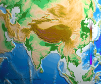
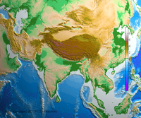
Sometimes it may happen that on a 3D image there is an apparent artifact line, look at the first figure on the right.
This is not an error, it is due to the fact that the interpolation function does not have data for the whole surface.
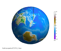
When developing the package, we found a simple remedy in adding a copy of the first column in the visualized data matrix at the end,
and also we add a copy of the first longitude value at the end.
For example, if you look at our TOPO elevation data, longitudes "lond_etopo2" are going from -180 till 180 deg,
and the first and last columns of "elev_etopo2_km" matrix are the same;
in this way, there is no line at the edge of the visualized elevation matrix
(see the second figure).
If the last duplicated column is deleted:
     lond_etopo2=lond_etopo2(1:end-1);
     elev_etopo2_km=elev_etopo2_km(:,1:end-1);
then an artefact line appears in the figure.
Have a look at this
script,
which demonstrates the problem and produces the two images shown.
|

|
Go to top
Any comments or questions will be appreciated – if you have some, please contact:
Ales Bezdek <>.
Last modified: 22 October 2020
|